Passive membrane

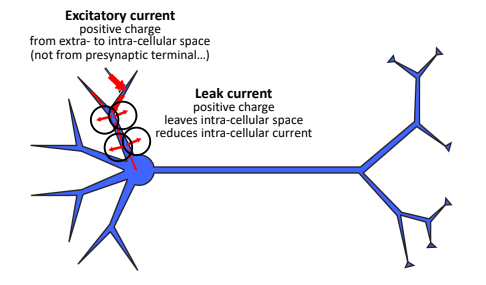
Synaptic currents

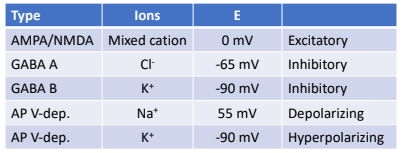
Ohmic conductances

The cable equation

Thanks to William Thomson (Lord Kelvin) we know if thin or thicc cables are better for the transatlantic telegraph.

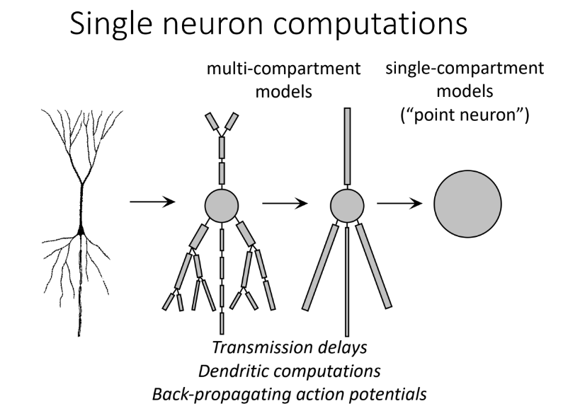
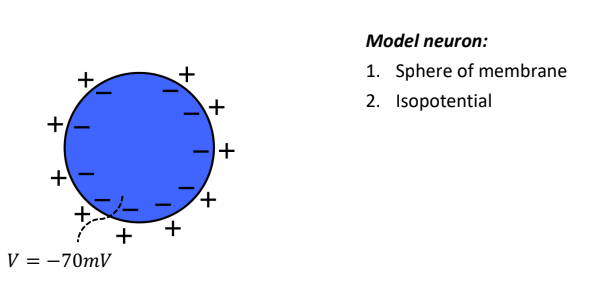
Single compartement model of a neuron

We use this model to derive a relation for the voltage of the neuron as a function of time $V(t)$.

Input resistance

Intuition

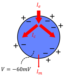
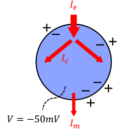
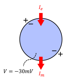
If we inject an external current $I_e$ into this neuron (ex: electrode), we will get a capacitive current $I_c$ that will dis/charge the membrane and depolarize the cell. That will lead to a leak current $I_m$ that will try to repolarize the cell.

Deriving $V(t)$

We will use the conservation of charge for this:
$$I_e = I_c + I_m$$
And Ohm's law to get $I_m$:
$$I_m = g_m(V-E_m)$$
And membrane capacitance to get $I_c$:
$$C_m = \frac{Q_m}{V} $$
$$C_m V = Q_m$$
By derivating relatively to time $t$ we get:
$$C_m \frac{dV}{dt} = \frac{dQ_m}{dt} = I_c$$
Plugging in to the first equation we get:
$$I_{e} - I_{m} = I_{c} $$$$I_{e} - g_{m}(V-E_{m}) = C_{m}\frac{dV}{dt}$$

Next using $g=\frac{1}{R}$, we can simplify to extract the time constant ($\tau = RC$):
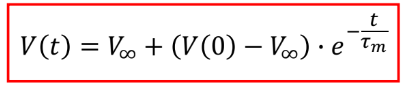
$$\begin{align}R_{m}I_{e}-(V-E_{m}) = \tau_{m} \frac{dV}{dt}\end{align}$$
where, $E_{m}$ is the resting potential

Steady state solution

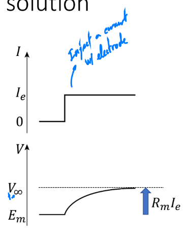
We can next solve this equation for a steady state solution, where we wait to infinity after an injection ($V = V(t=\infty) = V_{\infty}$):

This implies: $\frac{dV}{dt} = 0$
And we get:

$$\begin{align}R_{m}I_{e}-(V_{\infty}-E_{m}) = 0 \ \ V_{\infty} = R_{m}I_{e} + E_{m} \end{align}$$

General solution

Implications

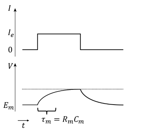
Time constant

1. Typically: $\tau_{m}$ ≈ 10 − 100ms
2. The time-scale of change in the cell (slow compared to a computer)
3. The short-term “memory” of the cell (short compared to an organism)
4. Activity “forgotten” after $\tau_{m}$
5. Longer memory: other mechanisms (e.g. plasticity, ...)
6. Slower response: recurrent connectivity (“reverberating activity”)

Spatial and temporal summation

Spatial summation

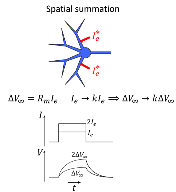
This is when different injections occur at the same time equally far away from the soma. This is a linear phenomenon, so doubling the current will double the potential.

Temporal summation

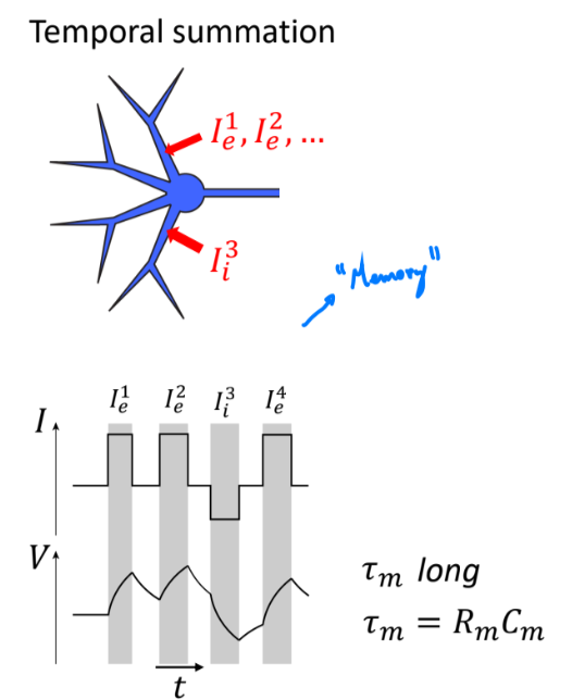
This is when inputs do not arrive at the same time but are nonetheless added. (not linear, it depends on the time constant)

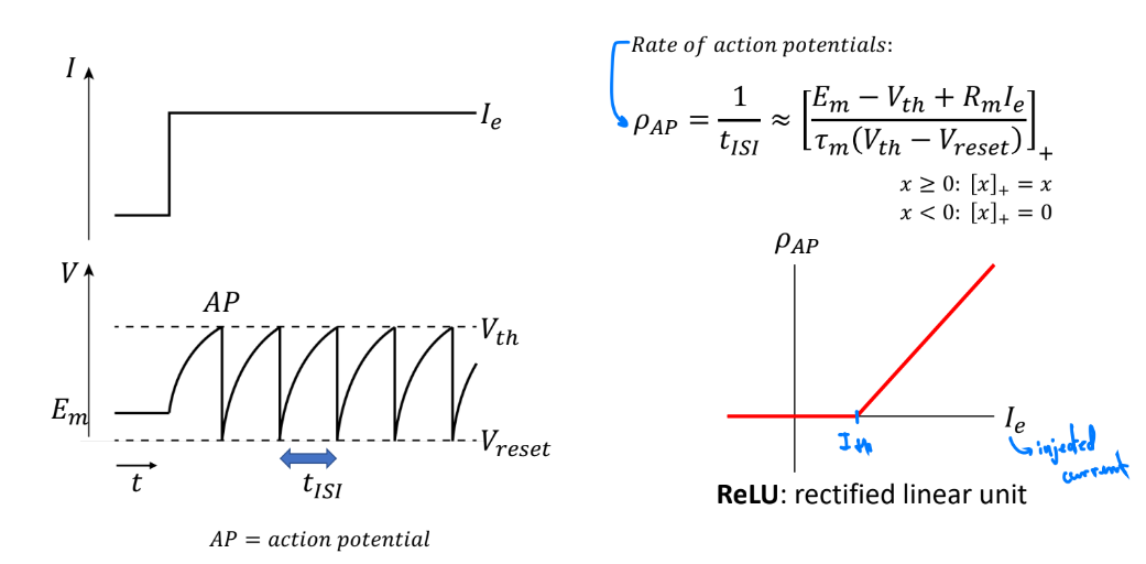
Integrate and fire neurons

Equivalent circuits

The following illustration shows the same as already mentioned above: There is an Input that will either flow in Capacitance and charge the membrane or go through the channels of the membrane.

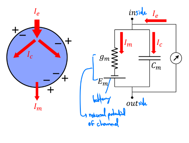
You could even add an additional channel type at the synapse ($I_{s}$) which is already open. The channel Is is excitatory since the positive part of the battery is on the inside, whereas $I_{m}$ is inhibitory.

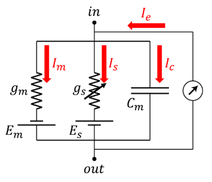
Using KCL we have:

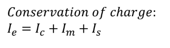
Plugging in the respective terms we get:
$$I_{e} = I_{c} + I_{m} + I_{s} $$
$$I_{e} = C_{m} \frac{dV}{dt} + g_{m}(V-E_{m})+g_{s}(V-E_{s}) $$
$$C_{m} \frac{dV}{dt} = I_{e} -g_{m}(V-E_{m})-g_{s}(V-E_{s})$$
At steady state $\frac{dV}{dt} = 0$:
$$V_{\infty} = \frac{I_{e}+g_{m}E_{m}+g_{s}E_{s}}{g_{m}+g_{s}}$$
If $I_{e}=0, \space g_{s} \gg g_{m}$:
$$V_{\infty} = E_{s}$$
If $I_{e}>0, \space g_{s} \gg g_{m}$:
$$V_{\infty} = E_{s} + \frac{I_{e}}{g_{s}}$$
(because $g_{m} \rightarrow 0$)
The last equation explains #shuntinginhibition: One synapse remains open and makes it harder for other synapses to increase the potential. (The effect of an external current is reduced by the $g_{s}$ conductance)

Deriving the full cable equation

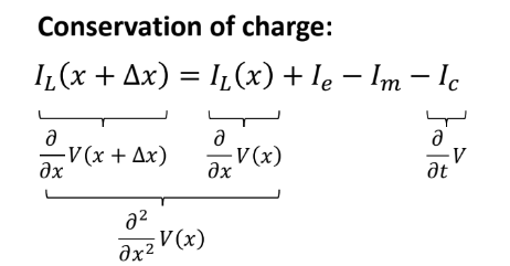
We start by adding longitudinal current and resistance.

Key assumption:
No cross current (orthogonal to x), ok for long distances.

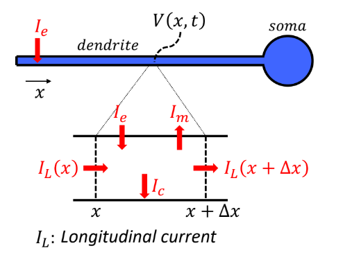
Applying conservation of charge:
$$\begin{align}I_{L}(x+\Delta x) = I_{L}(x) + I_{e} - I_{m} -I_{c}\end{align}$$

Longitudinal current

Makes the ==voltage change across space==

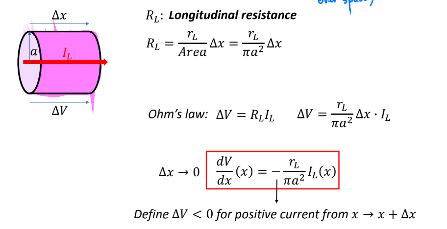
plugging in:

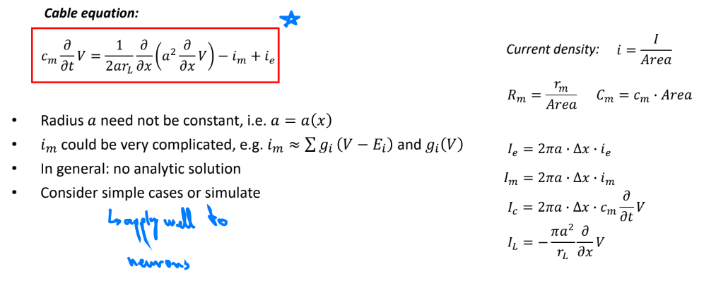
Cable equation

The cable equation has a function of time and space. To use it, the Radius a needs to be constant (you cannot have dendrites that get thinner and thinner). The variable $i_{m}$ could further get very complicated. In general, there is no analytic solution. That is why one needs to consider simple cases or simulate.

Linear cable equation

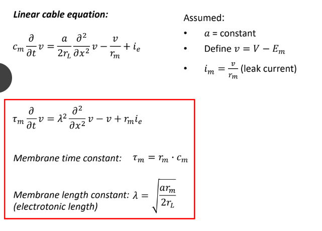
The time constant is how quickly things change over time.
The length constant is how quickly things change over space

Summary

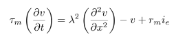
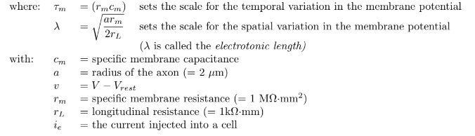
By injecting a constant current locally at $x=0$ the steady state solution is:

Cases

Infinite cable and constant current

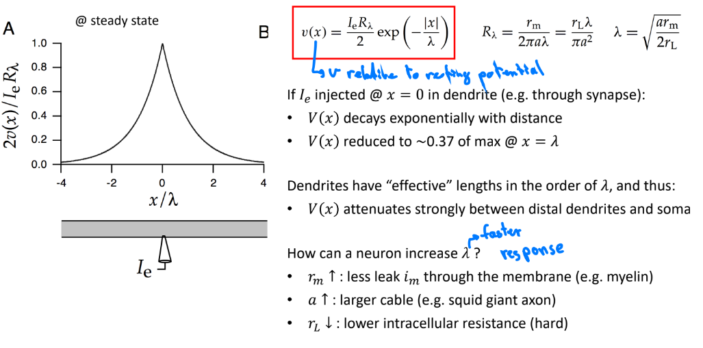
Panel A represents the fall-off over space

If $I_{e}$ injected @ $x=0$ in dendrite:
$V(x)$decays exponentially with distance
$V(x)$ reduced to $~0.37$ of max @ $x=λ$
$\rightarrow$ Voltage is highest at location where external current, then decays over space exponentially

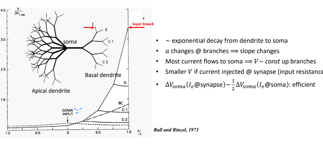
Dendrites have “effective” lengths in the order of λ and thus:
$V(x$) attenuates strongly between distal dendrites and soma

How can a neuron increase λ?
$r_{m}$ ↑: less leak im through the membrane (e.g. myelin)
$a$ ↑: larger cable (e.q. squid giant axon)
$r_{L}$ ↓: lower intracellular resistance (hard)

If λ increased, the potential will stay more constant $\rightarrow$ larger effect of a synapse into the soma

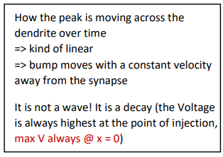
Infinite cable and current pulse (1 brief pulse)

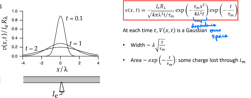
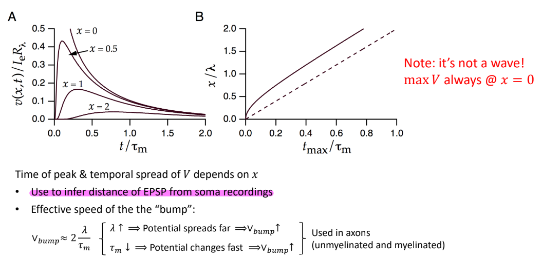
Passive currents in a branching neuron

Change my mind!