Hopfield networks
The Hopfield Network, or Hopfield Model, was proposed by John Hopfield in the early 80s. He was trying to understand what neural networks do. When we look into the brain and how neurons are connected to each other, we do not see always a clear pathway, i.e., it is hard to think about the connections in the brain in terms of input-output. He thought about connecting units to each other in an all-to-all pattern and see what would happen. It is a form of a recurrent neural network
Characteristics of hopfield networks
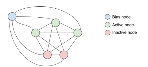
- Every nodes are interconnected but not to themselves (diagonal of adjacency matrix is $0$)
- Weights are symmetric ($W=W^T$) (due to hebbian synapse strengthening)
- Biais is a unit that is always on
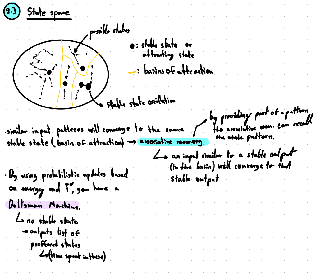
- Some states are stable and some are not. While in an unstable state, updating the network leads to a state change
- A stable state is a local minimum
Associative memory
We are used to think about computation as a process that receives an input, does something and generates an output. However, this is not what we “see” in the memory process, for instance. It seems our memory works with Pattern Completion, also known as Content Addressable Memory or Associative Memory. This memory has no input-output relation: given any piece of it, we can recover the rest. An example is when certain smell can bring us a memory, even though the smell is only part of the memory. Hopfield Networks can be used to give us insights about how the memory works by having a highly connected network that computes with no input-output, but with states. The network has some dynamics that ¨walk” through a state space, i.e., the space of all the possible states. The Hopfield Network is dynamic and moves from one state to another until it arrives to a stable state (also known as an attractor). Having stable states help the network to recover information giving partial inputs.
- A Hopfield Network is an associative type of memory. Information is stored in the stable states as local minima.
- It is important that information is distinct.
- Associative memory has room for error but is still recognizable. Convergence to nearby stable states.
- If some units are retrievable and all others are set randomly, the correct units will eventually set the wrong units right.
Dynamics of the model
- At each step, we chose a unit and update it's output
- The biais doesnt update
- $Q=$sum of all the active units weights. $Q$ always goes up or stays the same and a unit moves to an active status
- This means a hopfield network always converges to a stable state
- Like retrieving a memory
Greedy max Clique
Just our update algorithm. At each step, we chose a unit and update it's output.
Asynchronous update (doesn't match biology)
Depending on the unit we chose to start our updates with, we end up with a different stable state.
Synchronous update (doesn't match biology)
Let’s now consider a synchronous case, i.e., when we update all units at the same time: for this, active units for time t + 1 are computed based on active units at time t. In this case, the system becomes a deterministic system because it doesn’t depend on the order of updates anymore. Consider the network on Figure 41, starting with units 1 and 2 active, in the next step of update (after all units), unit 3 and 4 should be active. It may be confusing to see this by updating one unit per time, let’s say we update units in the order1, 2, 3, 4: after updating unit 3 it will become active but, when updating unit 4, we shouldn’t consider unit 3, yet.
To analyze a sychronous network, we consider a larger asynchronous network (for example two copies of the initial network linked together).
We converge to a cycling between a pair of steady states or one steady state.
Trick for analysis: make a larger asynchronous network based on the network we want to analyse. Duplicate the units in two columns and only use non-zero weights between them.
State space
From:https://github.com/benelot/eth-intro-to-neuroinformatics-summary