Feed forward networks

Feed-forward networks (FFN) are not like the networks in the brain. In the feed-forward networks, the information moves in only one direction (forward) from the input nodes, through the hidden nodes (if they exist), and to the output nodes. There are no cycles in this network. Usually, people are referring to feed-forward networks when they talk about artificial neural networks (ANN).

Structure

• Multiple layers of neurons with a certain number of inputs and outputs.
• Every layer of nodes feeds the next layer with inputs.
• Each input in one layer is connected to all the inputs in the next layer.
• There is an input and an output layer with hidden layers in between.

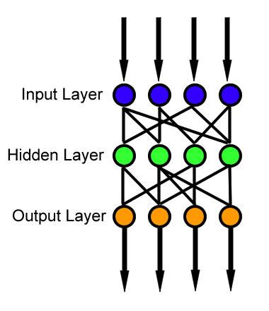
The weights are usually stored in a matrix ($W_{ij}$).

Why FFN are nice? Because we can think about functions that receive inputs and generate outputs. When we use FFN we know what we want to compute. We need to set the weights of the network in oreder to compute the function we want. The process of defining the weights is called learning or training. In feed-forward networks it is easy to evaluate each unit. The outputs are continuous functions of the input, which facilitates the optimization in case of wrong outputs. The training can be done using ”training data”: input/output pairs (xi , di). Where xi is the input value and di is the desired output. Then we can define the error $E = Σ_{k}(f(x_{k})−d_{k})^2$ , where $f(xk)$ is the output of the network. Differently of hopfield networks, we don’t need continuous updates and we do not reevaluate units. FFN have the idea of a pipeline (not like the brain). If a node on layer n in a FFN is connected to layer n + i with i > 1, this is still a FFN, however the most common structure is to connect nodes on layer n to nodes on layer n + 1. How can we change the weights to reduce the error? We can use gradient descent. We calculate all the $∂E/∂w_{i}$ in the network, easily, by starting at the end and then walking backwards. This is known as Backpropagation

Training process

1. Give to the network an input.
2. Calculate all the values in the network to produce the output.
3. Compare output with the desired output. This gives us the ”error” for this input.
4. Update the weights. For example, use gradient descent to optimize the parameters to minimize the error.

Backpropagation and Error function

• The inputs and desired outputs are given as $S={(x,d)^1,\ldots,(x,d)^l}$.
• The error function is given as $E(S) = \sum_i\frac{1}{2}||y(x^i)-d^i||^2$.
• The output is a non-linear transformation $y=f(a)$.
• $f(a)$ is the activation function, which is usually a sigmoid function.
• The error function for a single training sample is $E(S)=\frac{1}{2}(f(x_1w_1+x_2w_2+w_0)-d)^2$.
• The output of a simple network is for example $y(x_1,x_2,x_3)=f(x_1w_{21}+f(x_2w_{11}+x_3w_{12}+w_{10})w_{22}+w_{20})$.
• $\frac{\partial E(w_1,w_2,w_0)}{\partial w_1}=(f(x_1w_1+x_2w_2+w_0)-d)\cdot f'(x_1w_1+x_2w_2+w_0)\cdot x_1$.
• $\frac{\partial E(w_1,w_2,w_0)}{\partial w_2}=(f(x_1w_1+x_2w_2+w_0)-d)\cdot f'(x_1w_1+x_2w_2+w_0)\cdot x_2$.
• $\frac{\partial E(w_1,w_2,w_0)}{\partial w_0}=(f(x_1w_1+x_2w_2+w_0)-d)\cdot f'(x_1w_1+x_2w_2+w_0)$.

The error terms travel backwards through the network and get multiplied with the derivative of the activation function of that input. Multiple error terms can just be added up.

The partial derivative of the error $E$ term in relation to the weight $w$ to be adjusted can be added to the weight in order to learn. An additional weighting factor can be added.

Gradient descent

Consider $E = \sum(f_w(x) - y_i)^2$, we want to adjust $\vec{w}$ (weights of the network) to minimize $E$.

Gradient descent is the process of descending through the gradients (using the derivatives calculated with backpropagation), in this algorithm we try to reach the minimum of the loss function.

This is an iterative process.

Generally, the iterative process is given by $\theta_{i_{new}} = \theta_i + \Delta \theta_i$, where $\Delta \theta_i = - \alpha \frac{\partial J(\theta)}{\partial \theta_i}$.

No biological analogies have been found for now.

Change my mind!